Two Ways to Count Points in Polygons with R
How many bikes were stolen in your neighbourhood last year? The City of Ottawa reports individual bike thefts here, but it would be nice to have a fast way to aggregate those points into polygons so we can analyze and visualize them.
The rest of this post will work through this data to do just like it says on the tin: if you’ve got a set of points, you’ve got a set of polygons, and you’re using R, we’ll see two ways to count how many points are in each polygon.
Getting the Data
For this example we’ll use two spatial datasets from Ottawa’s incredible collection of open data. For our point data, we’ll use the set of bike thefts over the past several years. For our polygon data, we’ll use the most recent boundaries from the Ottawa Neighbourhood Study (ONS). (And for more maps and data, also check out the ONS’s website!)
Ottawa makes both of these datasets directly available in geojson format, so loading them is a snap using the sf package:
# load bike theft data
url <- "https://opendata.arcgis.com/datasets/3620cc7a3b874557bb288d889a4d56c2_0.geojson"
pts_online <- sf::read_sf(url)

# load ONS Gen2 shapefile
url <- "https://opendata.arcgis.com/datasets/32fe76b71c5e424fab19fec1f180ec18_0.geojson"
ons_online <- sf::read_sf(url)
A Brief Note about Mutually Exclusive & Collectively Exhaustive Sets
We’re assuming our polygon set is mutually exclusive and collectively exhaustive within our region of interest, which means that they cover all of it without overlapping.1 2 Fortunately, this is true for a lot of real-world spatial datasets like neighbourhoods, countries, or political ridings, so before using this code in your own projects just double-check that none of your own polygons overlap.3
Visualizing the Data
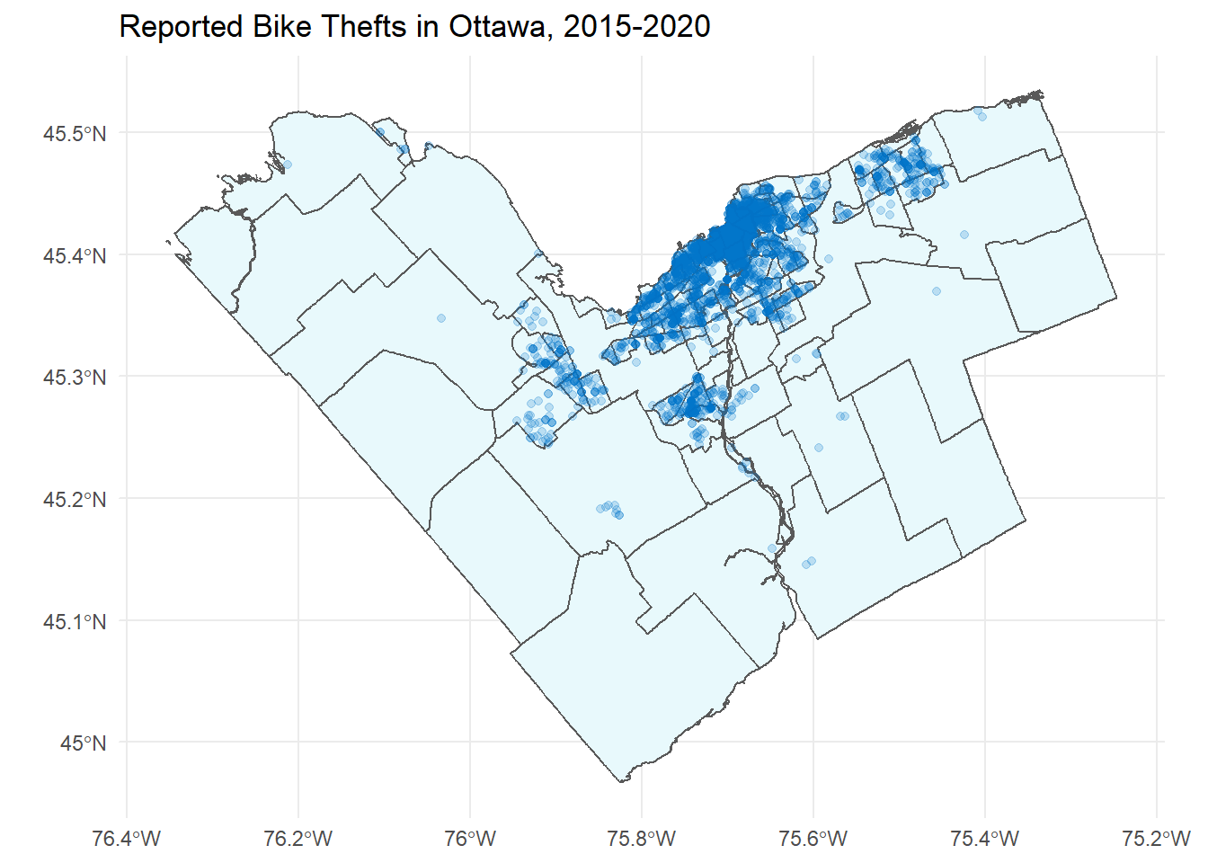
Visualizing your data is always a good first step, so here we’ll plot each theft on a map of Ottawa using a light transparency to see if bicycle thefts tend to cluster in certain areas. Not surprisingly, it looks like most thefts are concentrated in the more central regions, only a few thefts were reported in the Greenbelt (but more than none!), and there are pockets in Kanata, Barrhaven, and Orleans.
ggplot() +
  geom_sf(data = ons_online,
         fill = "#e8f9fc") +
  geom_sf(data = pts_online,
          colour = "#0074c8",
          alpha = 0.2) +
  theme_minimal() +
  labs(title = "Reported Bike Thefts in Ottawa, 2015-2020")
Since everything has loaded properly and looks sane, we can move on to the next step.
Method 1: Points First
We’ll start with the most versatile approach, which is to take each point and find out which polygon it’s in. The main function we’ll use is sf::st_join(), which takes two sf objects as inputs and returns an sf object containing the spatial join of our inputs. In plain(ish) English, if we give it a set of points and a set of polygons, it will return our set of points plus new data columns corresponding to the neighbourhood each point is in. It just works!
Let’s try it for our bike points and our neighbourhood polygons. Here we can see details for the first 10 reported thefts, each of which were in Old Barrhaven West.
sf::st_join(pts_online, ons_online) %>%
  sf::st_set_geometry(NULL) %>%
  select(ID, Incident_Date, Bicycle_Status, Name) %>%
  head(10) %>%
  knitr::kable(booktabs = TRUE,
col.names = c("ID", "Incident Date", "Bicycle Status", "Neighbourhood"))| ID | Incident Date | Bicycle Status | Neighbourhood |
|---|---|---|---|
| 1 | 08/02/2015 17:30 | STOLEN | Old Barrhaven West |
| 2 | 8/23/15 9:00 PM | STOLEN | Old Barrhaven West |
| 3 | 7/31/15 8:00 PM | STOLEN | Old Barrhaven West |
| 4 | 9/18/15 3:30 PM | RECOVERED | Old Barrhaven West |
| 5 | 11/13/15 5:30 PM | STOLEN | Old Barrhaven West |
| 6 | 5/18/16 8:50 AM | STOLEN | Old Barrhaven West |
| 7 | 6/28/16 9:00 AM | STOLEN | Old Barrhaven West |
| 8 | 05/07/2016 14:00 | STOLEN | Old Barrhaven West |
| 9 | 07/10/2016 20:27 | RECOVERED | Old Barrhaven West |
| 10 | 7/31/16 1:45 PM | STOLEN | Old Barrhaven West |
This almost seems too easy, so to add some value here’s a function that wraps it in some minimal data validation:
# function to get the neighbourhood each point is in
get_pts_neighbourhood <- function(pts, pgon){
  # check input validity
  if (!"sf" %in% class(pts)) stop("Invalid input: pts must have class 'sf', e.g. a shapefile loaded with sf::read_sf().")
  if (!"sf" %in% class(pgon)) stop("Invalid input: pgon must have class 'sf', e.g. a shapefile loaded with sf::read_sf().")

  # make sure the two datasets have the same CRS
  if (sf::st_crs(pts) != sf::st_crs(pgon)) pts <- sf::st_transform(pts, sf::st_crs(pgon))

  # do a spatial join
  results <- sf::st_join(pts, pgon)

  return (results)
}
With this function in hand, counting the number of points is then just a matter of piping to dplyr::summarise() as follows:
get_pts_neighbourhood(pts_online, ons_online) %>%
  sf::st_set_geometry(NULL) %>%
  group_by(Name) %>%
  summarise(num = n()) %>%
  arrange(desc(num)) %>%
  head(10)  %>%
  knitr::kable(booktabs = TRUE,
col.names = c("Neighbourhood", "# Thefts"))| Neighbourhood | # Thefts |
|---|---|
| Centretown | 1113 |
| Sandy Hill | 710 |
| Glebe - Dows Lake | 324 |
| Byward Market | 278 |
| West Centretown | 209 |
| Westboro | 179 |
| Carleton University | 161 |
| Overbrook - McArthur | 133 |
| Hintonburg - Mechanicsville | 132 |
| Laurentian | 111 |
We won’t delve into the data too much, but this looks plausible: the most thefts were reported in downtown areas with lots of bars, restaurants, and universities, just where we might expect there to be more bikes and more bike thefts.
Method 2: Polygons First
The second way of counting is to jump straight to the polygons without locating each point. As a bonus, it’s more complicated and less versatile! You don’t get point-level data, but if you only care about aggregating points into polygons then that’s not a problem.
The main function we’ll use is sf::st_intersects(), which takes two sf objects as inputs and returns a sparse geometry binary predicate (SGBP) list.
sf::st_intersects(ons_online, pts_online) ## Sparse geometry binary predicate list of length 111, where the predicate was `intersects'
## first 10 elements:
## 1: 1, 2, 3, 4, 5, 6, 7, 8, 9, 10, ...
## 2: 32, 33, 34, 35, 36, 37, 38, 39, 40, 41, ...
## 3: 1513, 1514, 1515, 1516, 1517, 1518, 1519, 1520, 1521, 1522, ...
## 4: 2966, 2967, 2968, 2969, 2970, 2971, 2972, 2973, 2974, 2975, ...
## 5: 2246, 2247, 2248, 2249, 2250, 2251, 2252, 2253, 2254, 4104
## 6: 4482, 4483, 4484, 4485, 4486, 4487, 4488, 4489, 4490, 4491, ...
## 7: 4175, 4595, 4596, 4597, 4598, 4599, 4600, 4601, 4602
## 8: 5351, 5354, 5360, 5557, 5558, 5560
## 9: 5474, 5475, 5476, 5477, 5478, 5479, 5480, 5481, 5482, 5483, ...
## 10: 5139, 5140, 5141, 5142, 5143, 5144, 5145, 5146, 5147, 5148, ...We have one element of our SGBP list for each neighbourhood, and each list element holds the row indices of the points that are inside of it.To get the number of points in each polygon we need the number of indices in each list element, which we can get by piping our SGBP list into lengths().
sf::st_intersects(ons_online, pts_online) %>%
  lengths()
With some piping, we can mutate() these numbers into a new column in our original polygon data. If we were to wrap it all up in a function with some basic validation, it might look like this:
# function to count the number of points in each polygon.
group_by_neighbourhood <- function (pts, pgon) {
  # check input validity
  if (!"sf" %in% class(pts)) stop("Invalid input: pts must have class 'sf', e.g. a shapefile loaded with sf::read_sf().")
  if (!"sf" %in% class(pgon)) stop("Invalid input: pgon must have class 'sf', e.g. a shapefile loaded with sf::read_sf().")

  # make sure the two datasets have the same CRS
  if (sf::st_crs(pts) != sf::st_crs(pgon)) pts <- sf::st_transform(pts, sf::st_crs(pgon))

  # count the number of points in each polygon
  results <- pgon %>%
    mutate(num = sf::st_intersects(pgon, pts) %>% lengths()) %>%
    select(-geometry, geometry)

  return (results)
}
And we could test it like so:
group_by_neighbourhood(pts_online, ons_online) %>%
  sf::st_set_geometry(NULL) %>%
  select(Name, num) %>%
  arrange(desc(num)) %>%
  head(10)  %>%
  knitr::kable(booktabs = TRUE,
col.names = c("Neighbourhood", "# Thefts"))| Neighbourhood | # Thefts |
|---|---|
| Centretown | 1113 |
| Sandy Hill | 710 |
| Glebe - Dows Lake | 324 |
| Byward Market | 278 |
| West Centretown | 209 |
| Westboro | 179 |
| Carleton University | 161 |
| Overbrook - McArthur | 133 |
| Hintonburg - Mechanicsville | 132 |
| Laurentian | 111 |
This gives us the same results as Method #1, just using a few more function calls. (Although before finding st_join() I was using an even more convoluted method, so I’m not one to judge.)
So where are the most bicycle thefts?
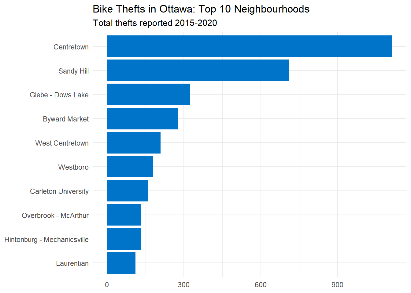
It would be a shame to do this work without any visualizations! Here we’ll use our point-first approach and then some dplyr magic to count the number of thefts in each neighbourhood. Centretown is at the top of the list, but a few other downtown neighbourhoods also have strong showings. After that, thefts drop off exponentially and there’s a long tail of neighbourhoods (not shown here) with few or no thefts.
get_pts_neighbourhood(pts_online, ons_online) %>%
  sf::st_set_geometry(NULL) %>%
  group_by(Name) %>%
  summarise(num = n()) %>%
  arrange(desc(num)) %>%
  head(10) %>%
  ggplot() +
  geom_col(aes(x = reorder(Name, num), y=num),
           fill = "#0074c8") +
  coord_flip() +
  theme_minimal() +
  labs(x = NULL,
       y = NULL,
       title = "Bike Thefts in Ottawa: Top 10 Neighbourhoods",
       subtitle = "Total thefts reported 2015-2020")
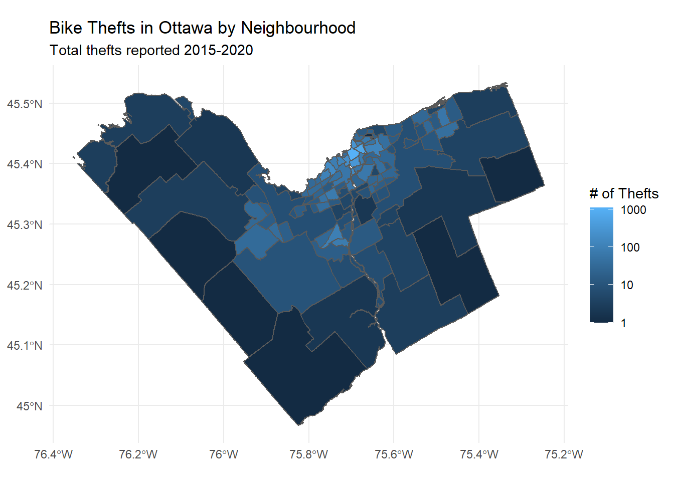
Since we have geospatial data, we can also use our polygon-first approach to see how it looks on a map if we shade each neighbourhood based on how many thefts it had. Again we can see the brightest spots right downtown, with some brighter patches for Kanata, Barrhaven, and Orleans, and dark patches in more rural neighbourhoods. Note that I’ve used a logarithmic scale here with scale_fill_gradient() (thanks to this tip) to make the detail more apparent.
group_by_neighbourhood(pts_online, ons_online) %>%
  ggplot() +
  geom_sf(aes(fill = (num+1))) +
  theme_minimal() +
  labs(title = "Bike Thefts in Ottawa by Neighbourhood",
       subtitle = "Total thefts reported 2015-2020",
       fill = "# of Thefts") +
  scale_fill_gradient(trans = "log",
                      breaks = c(1, 10, 100, 1000, 1500),
                      labels = c(1, 10, 100, 1000, 1500))
Summary
We’ve used two methods to assign points to polygons: a versatile point-first approach using sf::st_join(), and a polygon-first approach using sf::st_intersects(). We developed some simple wrapper functions for basic data validation, and then applied these functions to some real-world data from the City of Ottawa.
Was this useful/wrong/overly convoluted? Let me know your thoughts!
To be precise, I’m assuming the polygons overlap only along their borders. But since this is a set of measure zero, we can assume such an event has probability zero and safely ignore it.↩︎
And here I advance the following conjecture: when doing data science, the probability of an error arising in theory is inversely proportional to the probability of it arising in practice.↩︎
You could imagine overlapping polygons being common in some disciplines, for example if you were mapping regions where various languages are spoken in the home.↩︎