Three Kinds of Websites

First we need to distinguish between three types of websites: static, dynamic server-side, and dynamic client-side. Each site types needs a different web-scraping approach, which we’ll discuss using a strained metaphor based on men’s fashion.

Static sites are like off-the-rack suits: everyone gets the same thing. They consist of a bunch of static files (html, images, css, and so on) that live on a web server that your browser loads and interprets. For example, this blog is a static website rendered using Blogdown and Hugo.. You can scrape static sites in R using rvest to load and parse the sites, and Selector Gadget to find the css or xpath for the features you’re interested in.

Dynamic server-side sites are like made-to-measure suits: they’re customized at the point of origin based on your needs and requests, and everyone gets something a bit different. The html is generated dynamically on a server, maybe using a programming language like php, and then sent to your browser. You can scrape these sites using Selenium to load them in a browser and extract the data (see this blog post for details).

Dynamic client-side sites are a bit like an outsourced made-to-measure suit, where the fabric is measured and cut somewhere else and then shipped to you to be sewn together. (The metaphor is now broken and will be discarded.) This means that the remote server sends structured information to your browser, which then builds a nice html file and shows to you. The idea behind API interception is that we can ask for the structured data ourselves, without the need to work backwards from the final html file. When it works, this can be very efficient.

Step 1: Use the Google developer console to find the API call(s)

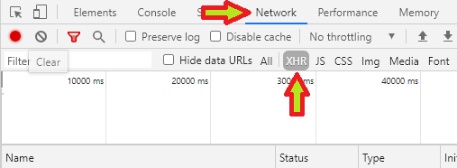
First, assuming you’re using Chrome on Windows, open the developer console by pressing Ctrl-Shift-J. A new frame should pop open. Within that frame, Click Network on the top bar and then XHR below that.¹ Here’s an image with helpful and unmissable arrows:

Now load the site you’re interested in: here I’ll be using the Ontario Newsroom. You should see a bunch of rows added to the developer console, like this:

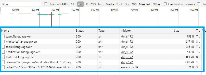
These are all the API calls that our browser made to Ontario’s severs to generate the web page we’re now looking at.

Next we need to figure out which of these API calls we’re interested in. Some sites can have dozens, so this isn’t always easy. Sorting by size can be helpful, since bigger responses might mean more useful data. In the image above you can see that featured?language=en and releases?language=en... are both pretty big, so let’s focus on them.

If you click an API call’s name Chrome will show more information, and you can click in the new sub-tab that opens up to get different views. We care mostly about Headers, Preview, and Response, and if we click on Preview Chrome will give us a structured view of the response. If we click on featured?language=en, and then on Preview, we get the following:

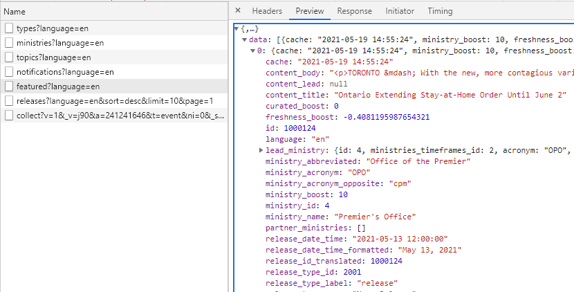
This looks very promising! The data on the right matches the featured release on the web page! So it looks like this API call gives us the current features press releases in a nice structured format: you can see that it gives us the text in content_body, the release_date_time, the lead_ministry, and a bunch of other stuff too. So if you wanted to make an app that shows the current top-priority government press releases, this is what you could use. You can also view the results in your browser, although they’re a bit messy.

But we want to get as many news releases as we can, not just the featured ones, so we need to keep looking. Then next one, releases, looks like it might have what we’re looking for:

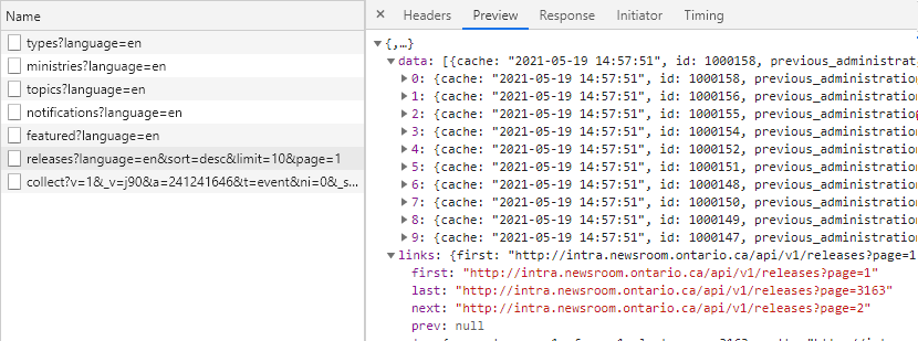
Yes! Here we see 10 responses under data, and if we click through we’ll find one entry for each of the 10 press releases loaded in our browser. Let’s also take note of that one line under links that says last: "http://intra.....?page=3163. Perhaps there are 3163 pages of results!

Step 2: Reverse-engineer the API calls

Now that we’ve found the right API call, the next step is to reverse-engineer it so that we can get the data we want. This is can be a tricky trial-and-error process. Sometimes you’ll need to navigate around a web page for a few minutes and track the API calls to figure out what’s going on, but the Ontario Newsroom API is straightforward. Let’s break it down:

https://api.news.ontario.ca/api/v1/releases?language=en&sort=desc&limit=10&page=1

• https://api.news.ontario.ca/api/v1/releases: This is API endpoint, or web address. The question mark then tells the API that everything after that point is parameters.
• language=en: We can pretty safely assume that this tells the API to give us results in English.
• sort=desc: This seems like it’s telling the API to sort results in descending order, which might mean to put the most recent press releases first.
• limit=10: There were 10 press releases on the web page, so this might tell the API how many results to return. This one’s interesting.
• page=1: We’re on the first page of releases, so this might tell the API which releases to return. This one’s interesting too.

At this point I’ll usually fire up RStudio and start querying the API with different parameters. With three lines of code, we can query the API and parse the results:

library(tidyverse)
library(httr)

response <- httr::GET(url = "https://api.news.ontario.ca/api/v1/releases?language=en&sort=desc&limit=10&page=1")

response_json <- httr::content(response, type = "application/json", encoding = "UTF-8")

And it works!

But wouldn’t it be nice to get more than 10 at a time? Why not go for something bigger, like 500? It’s simple enough to try: just put limit=500 in the API request:

response <- httr::GET(url = "https://api.news.ontario.ca/api/v1/releases?language=en&sort=desc&limit=500&page=1")

response_json <- httr::content(response, type = "application/json", encoding = "UTF-8")

And it also works! Some APIs will oblige but others will choke if you ask for too much at once, so you may need to experiment. I’m not sure if it’s better manners to make more requests that are smaller or fewer that are larger, but it’s easier for us to make fewer calls.

Step 3: Call the API and store the results.

Now that we’ve found the API and we know how it works, we can use a simple loop to call it as many times as we need to. I’m going to store all the results verbatim in a list and parse them in step 4, but for simple results you could parse the results as you get them.

I’ve checked the response metadata and it says there are 64 pages of 500 results each, so here we’ll call the API 64 times and save the results in a list.

Please be polite when calling these APIs, for example by including some built-in delays between calls so you don’t spam the host server. The rvest package authors have written some best practices for API packages and it’s a good idea to follow them as closely as possible.

results <- list()

for (i in 1:64){
  message(paste0(i,"/64"))
  url_i <- paste0("https://api.news.ontario.ca/api/v1/releases?language=en&sort=desc&limit=500&page=",i)
  results[[i]] <- httr::GET(url = url_i)
  
  Sys.sleep(1) # Pause politely
}

Step 4: Tidy the Data

In this final step we parse the API’s responses and put them into a usable format. This is an art, not a science, but I like to use a tidy format whenever possible because it’s easy to work. I also try not to use nested tibbles for storage, so that my data is maximally shareable in csv files.

If you do use a tidy unnested format, you’ll need to decide what to do with nested columns that contain lists of varying lengths. In this data set, some releases have no quotes and some have ten, and some have one topic and some have five. To keep it simple I’ve compressed them down into character vectors, but keeping enough structure that I can parse them back out into nested tibbles if I need to.

This next code block does the wrangling and tidying:

# This is where our results will go once we tidy them up.
results_parsed <- tibble::tibble()

# A humble for-loop to parse each of our results.
# This is definitely not memory optimized: I'm using bind_rows() to add new data to old data.
# If you have millions of rows you'll want to be smarter about this.
for (i in 1:length(results)){
  message(paste0(i,"/",length(results)))
  
  # Get the i-th result
  r <- results[[i]] %>%
    httr::content(type = "application/json", encoding = "UTF-8")

  # Wrangle it into a tidy format.
  # This is long & complex but I built it step by step, basically guessing and checking.
  # Note: because we don't know how many quotations there are, I've put that column into a json string.
  result <- r$data %>% 
    enframe() %>%
    mutate(value =  purrr::map(value, enframe)) %>%
    mutate(value = purrr::map(value, pivot_wider)) %>%
    unnest(value)  %>%
    mutate(topics = purrr::map(topics, function (x) purrr::map(x, pluck, "label")) %>% purrr::map(stringr::str_flatten, collapse = " | ") %>%
             unlist() ) %>%
    mutate(tags = purrr::map(tags, function (x) purrr::map(x, pluck, "label")) %>% purrr::map(stringr::str_flatten, collapse = " | ") %>%
             unlist() )%>%
    mutate(partner_ministries = purrr::map(partner_ministries, function (x) purrr::map(x, pluck, "acronym")) %>% purrr::map(stringr::str_flatten, collapse = " | ") %>%
             unlist() ) %>%
    mutate(quotes = purrr::map(quotes, jsonlite::toJSON)) %>%
    select(id, contacts, content_title, content_subtitle, content_lead, content_body, keywords, media_assets, ministry_id, ministry_acronym, ministry_name, partner_ministries, quotes, quickfacts, release_date_time, release_id_translated, release_type_id, release_type_label, release_crossreferences_resources, release_resources, slug, topics, distributed) %>%
    mutate(across(everything(), as.character))%>%
    mutate(across(everything(), function(x) if_else(x == "NULL", "", x)))
  
  results_parsed <- bind_rows(results_parsed, result)
} 

write_csv(results_parsed, "ontario_newsroom.csv")

And that’s it! It might seem silly to say, but don’t forget to save your results! You may want to save the tidy data as a .csv file and the original raw results in an .RData file in case you want to go back to it later.

Is There a Friday-Afternoon News Dump?

After all this work collecting data, I feel a strong need to answer a trivial question. So I ask: is there any truth to the idea of a “Friday afternoon news dump?” I’ve heard anecdotal suggestions that bad news tends to be announced late on a Friday when people are less likely to notice, but now we have a dataset of 31,649 news releases spanning nearly 15 years that we can use to take a look.

First, let’s just look at the days of the week:

weekdays <- results_parsed %>%
  select(release_date_time) %>%
  mutate(release_date_time = lubridate::ymd_hms(release_date_time)) %>%
  mutate(day_of_week = lubridate::wday(release_date_time, label = TRUE)) %>%
  group_by(day_of_week) %>%
  summarise(num = n())

forplot <- weekdays %>%
  ggplot(aes(x=day_of_week, 
             y = num,
             text = paste0("Weekday: ", day_of_week,
                           "\nCount: ", num))) +
  geom_col(fill = "#123456") +
  theme_minimal()  +
  labs(title = "Ontario Press Releases, July 2007 - May 2021",
       subtitle = "Grouped by Day of the Week",
    x = "Day of Week",
       y = "# of Releases")

plotly::ggplotly(forplot, tooltip = c("text")) 

It’s not an overwhelming “dump,” but it does look like more news releases come out later in the week.

This still doesn’t answer our question though, because we wanted to know if more releases come out on Friday afternoon. The next plot shows the percentage of daily press releases that were issued at each hour of the day for each day of the week. To keep it simple I’ve removed releases that didn’t specify a time (otherwise they showed up at midnight, 0 o’clock), and removed Saturday and Sunday to keep it simple.

weekdays_hours <- results_parsed %>%
  select(release_date_time) %>%
  mutate(release_date_time = lubridate::ymd_hms(release_date_time)) %>%
  mutate(day_of_week = lubridate::wday(release_date_time, label = TRUE),
         hour = lubridate::hour(release_date_time)) %>% 
  filter (hour > 0) %>%
  group_by(day_of_week, hour) %>%
  summarise(num = n())

forplot <- weekdays_hours %>%
  filter(!day_of_week %in% c("Sat", "Sun") ) %>%
  group_by(day_of_week) %>%
  mutate(pct = num / sum(num)) %>%
  ggplot(aes(x=hour, 
             y = pct,
             fill = day_of_week,
             text = paste0("Weekday: ", day_of_week,
                           "\nHour: ", hour,
                           "\nPercent: ", (round(pct, digits = 3) * 100) ,"%"))) +
  geom_col(position = "dodge") +
  theme_minimal()  +
  labs(title = "Ontario Press Releases, July 2007 - May 2021",
    x = "Hour of the Day",
       y = "% of Releases",
    fill = "Weekday") +
  scale_y_continuous(label = scales::percent)

plotly::ggplotly(forplot, tooltip = c("text"))

We get a nice bimodal distribution with peaks at around 10am and 2pm, and some oddly long tails which might be neat to look into. To answer our question, yes, it does look to me like Friday has a slightly elevated bar at hour 16, 4pm, especially compared to Thursday. And Friday’s percentages at other times are quite a bit lower than those of the other days. So there’s some rough evidence for a Friday afternoon news dump.

The bigger surprise to me is that there’s stronger evidence of a Friday morning news dump! Friday’s bars at 10am and 11am tower over its neighbours.

There’s lots more to look into here, of course, but this gives a sense of what’s possible (and why we might want to go to the trouble of getting this kind of data.)

Summary

This post introduced a new web-scraped technique called API interception, which can give direct access to the structured data behind some modern dynamic web sites. We walked through a case study using the Ontario Newsroom and outlined the four main steps to using this technique. We then made some simple plots to see whether there’s evidence of a “Friday news dump” in Ontario, and we found some evidence that more news stories are released on Friday mornings.

Once you have the process down the code only takes a few minutes to run. It’s pretty amazing, because when I tried using Selenium it took hours to get only a fraction of the data.

You can grab the data here in two ~75 meg files (file #1, file #2). This data is © Queen’s Printer for Ontario, 2007-2021, and I’m providing it for educational and non-commercial purposes with full credit and acknowledgement consistent with the Newsroom’s copyright information page.